Calibration of a diffraction setup using the Graphical User Interface (GUI)#
Here is the cookbook which will explain you how to calibrate the setup of a diffraction experiment within five minutes. No advanced features are presented.
Video#
The graphical tool for geometry calibration is called pyFAI-calib2,
just open a terminal and type its name plus return to start up the application
which looks like this:
$ pyFAI-calib2
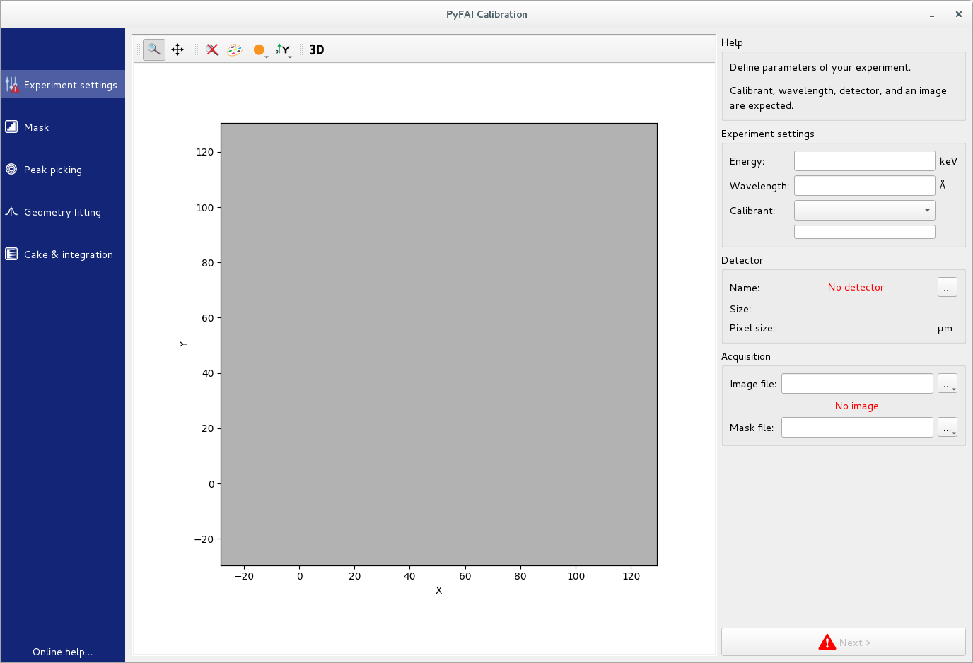
The windows is divided in 3 vertical tiles (panels) containing:
On the left side, a list of tasks to be performed: setting-up, masking, peak-picking, ring-fitting and caking.
A large central panel to display the image. Note the zoom, pan and colormap buttons on the top of the central panel.
The right side panel contains a set of tools dedicated to each task and finishes with the
Nextbutton to switch to the next task.
We will now describe shortly every task by following a simple example.
Experiment settings#
This task contains all entries relative to the experiment setup. It is the place where you can enter the energy of the beam (or the wavelength), the calibrant and the detector used.
You have to provide the calibration image which is then displayed in the central panel.
For example the file used in this cookbook can be downloaded from this link:
Eiger4M_Al2O3_13.45keV.edf.
Click on the ... on the right of Image file to open the file-browser
which will allow you selecting the file you just downloaded.
Finally, select the type of detector, here the image has been acquired using an Eiger4M manufactured by Dectris. Once the detector is selected, its shape is overlaid to the image allowing a direct validation of the detector size. Mask and dark-current files can be provided in a similar way.
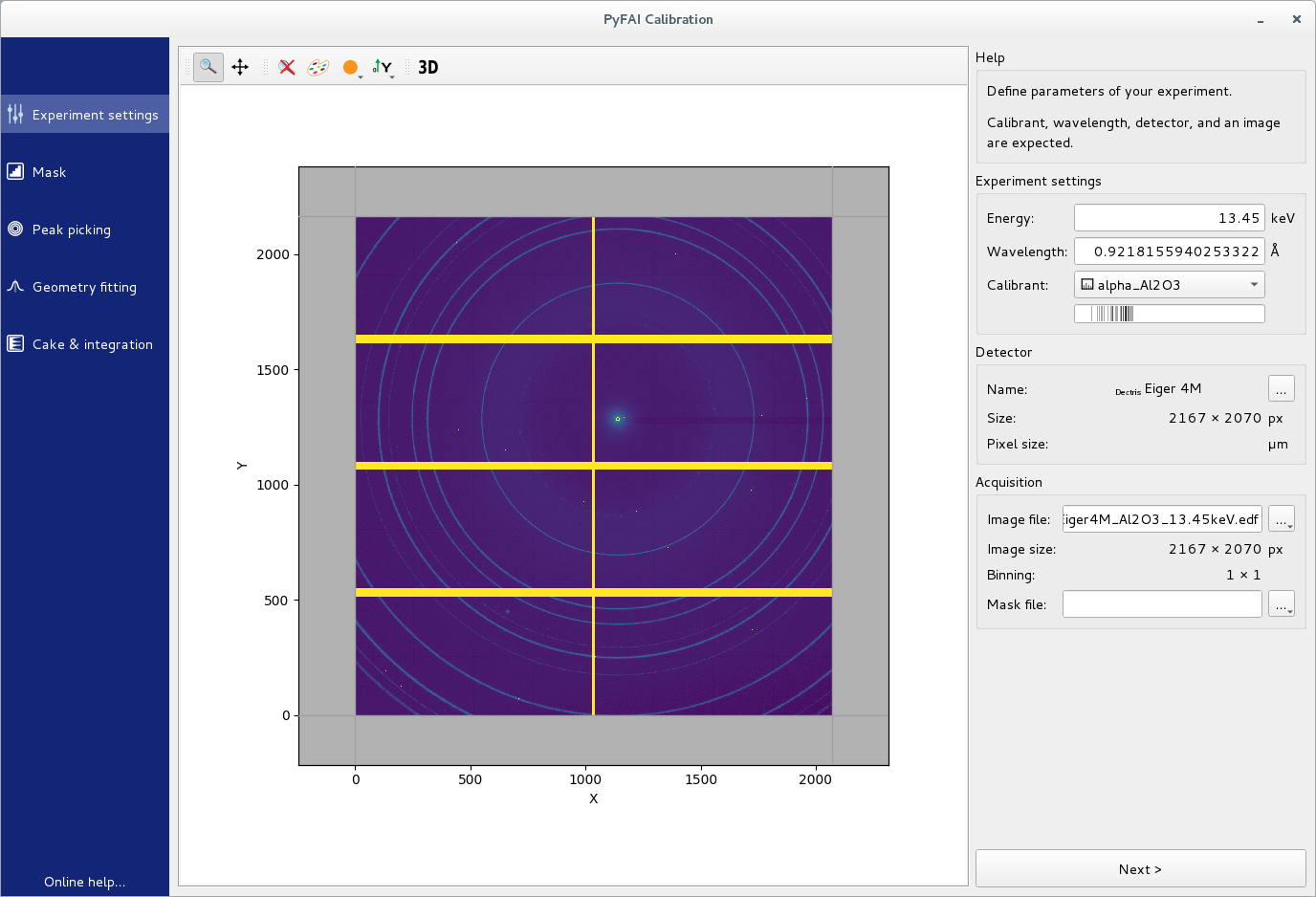
Finally set the energy of the experiment (or the wavelength) and select the
reference compound used in the calibrant drop-down menu.
For this image, the beam was at 13.45 keV and the calibrant was corundum, which
is referenced alpha_Al2O3 as in the figure.
You are now ready to define the mask, click on the Next> button.
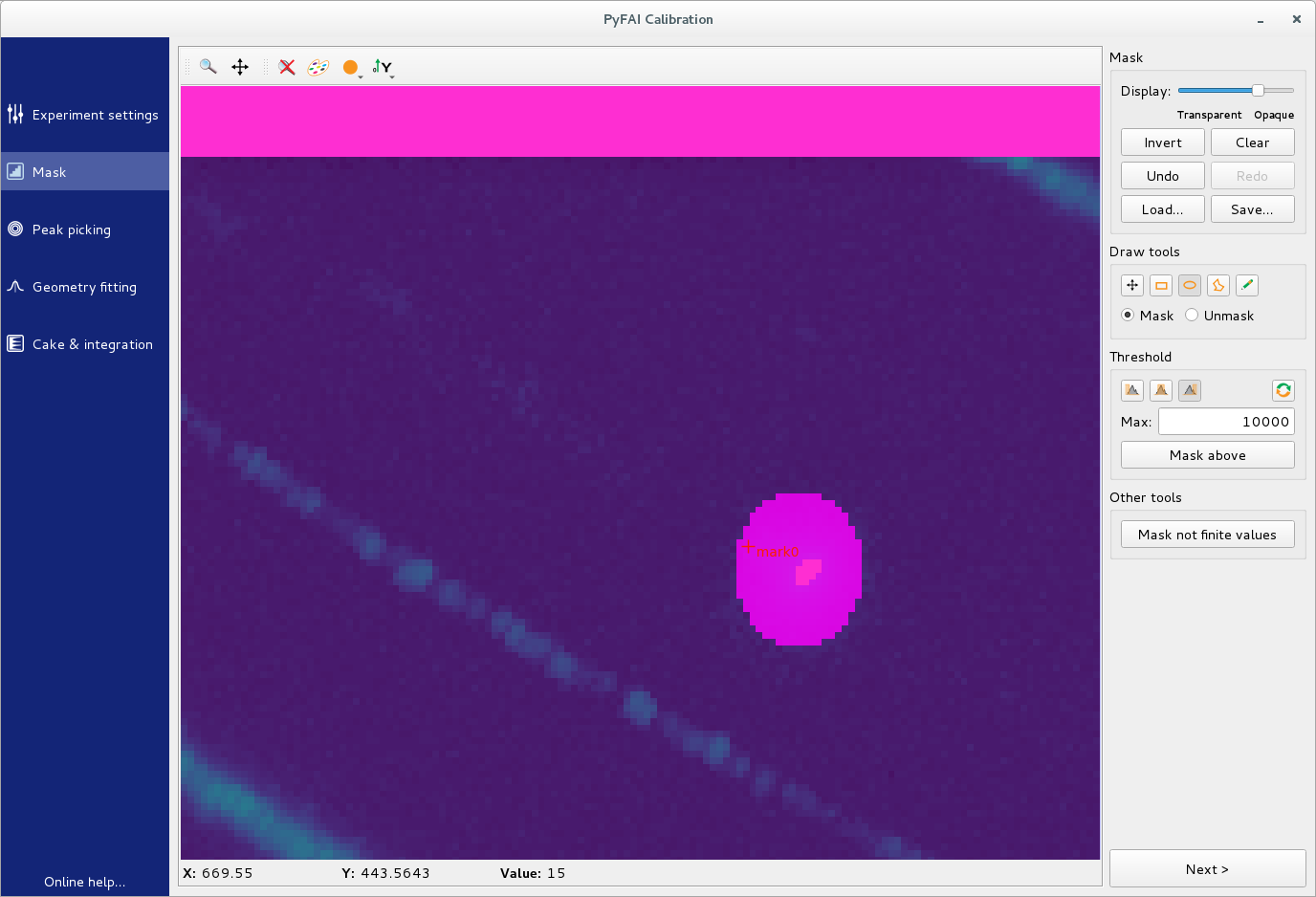
Defining the mask#
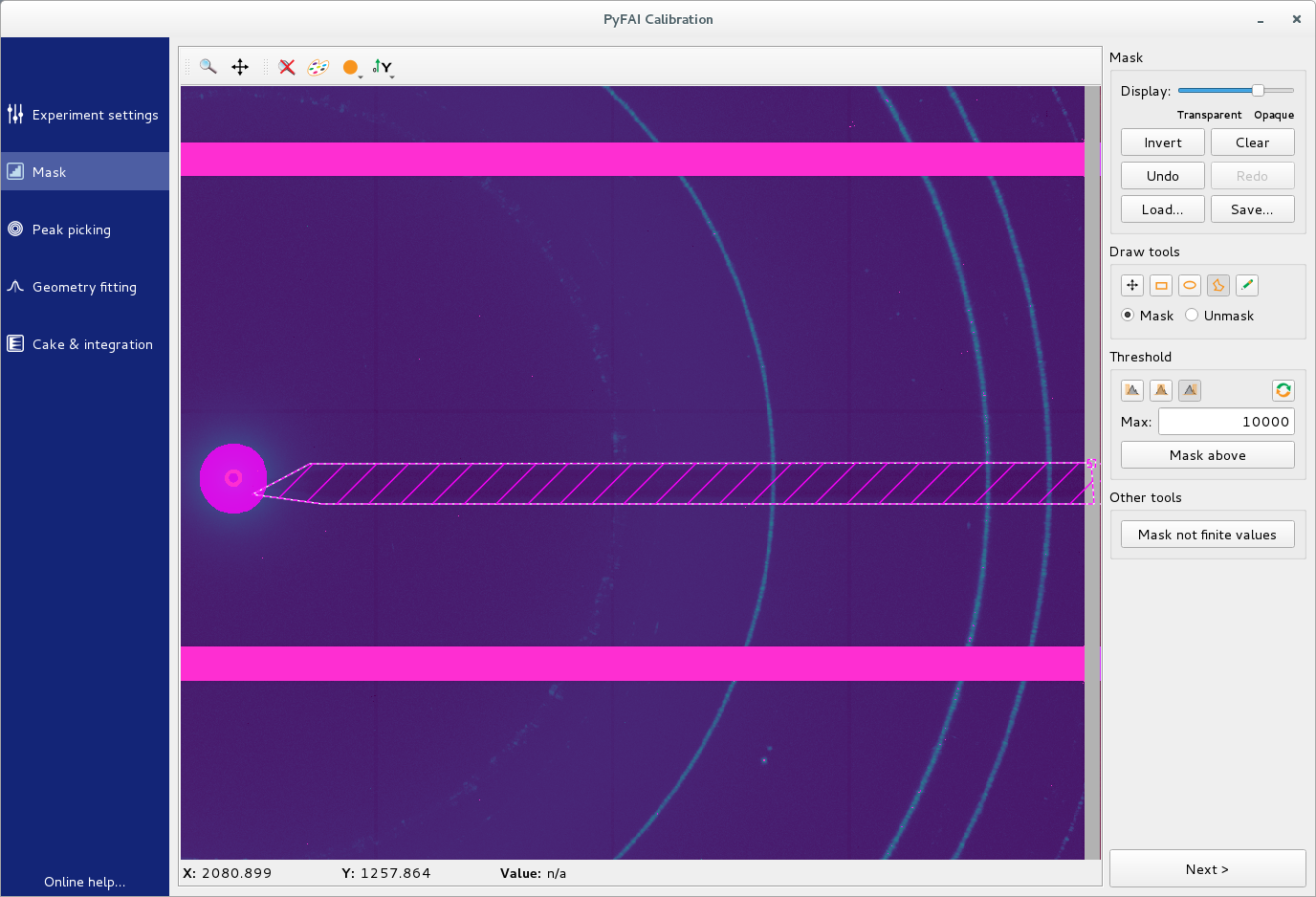
The mask defines the list of pixels which are considered invalid. It is displayed in green by default. There are 3 drawing tools:
rectangular selection
polygonal selection (click on the first point to finish edition)
pencil selection
In addition, the mask can often be setup easily using one or two thresholds, or by discarding infinite values or NaN. Finally, masks can be inverted, saved and restored.
In our test-image, the Eiger detector has flagged overflow pixel with a very high value. Discarding pixel values above 65000 removes automatically all invalid pixels. To remove pixels with some shadow, like the beam stop, the easiest is to use the polygon tool (click on the square of the first point to finish the edition) as in the figure below:
Once you are done, click on the Next> button to pick some rings.
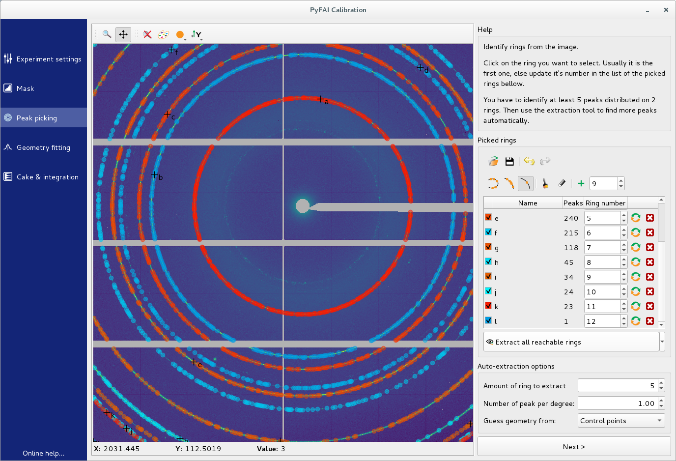
Peak-picking and ring assignment#
The geometry calibration is performed in pyFAI by a least-square fitting of peak positions on ring number.
This task consists in selecting groups of peaks by left-clicking on them in the image, and to assign the proper ring number to each group.
You will need to pick at least two rings. Selecting the inner-most (2 or 3) rings is advised as they are the most intense and misassignment is unlikely.
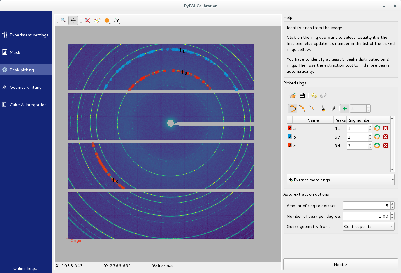
Double check the ring-number assignment in the right panel. In the case of a difficult image (discontinuous rings, spotty signal, …), changing the picking mode can help.
Nota: this GUI tool uses 1-based numbers, unlike the command line tool which starts at 0.
We will skip the Recalibrate tool for now and go directly to the
geometry fitting by clicking on the Next> button.
Geometry fitting#
When arriving on this task, the geometry is immediately fitted and you can see the values of the 3 translation and 3 rotation.
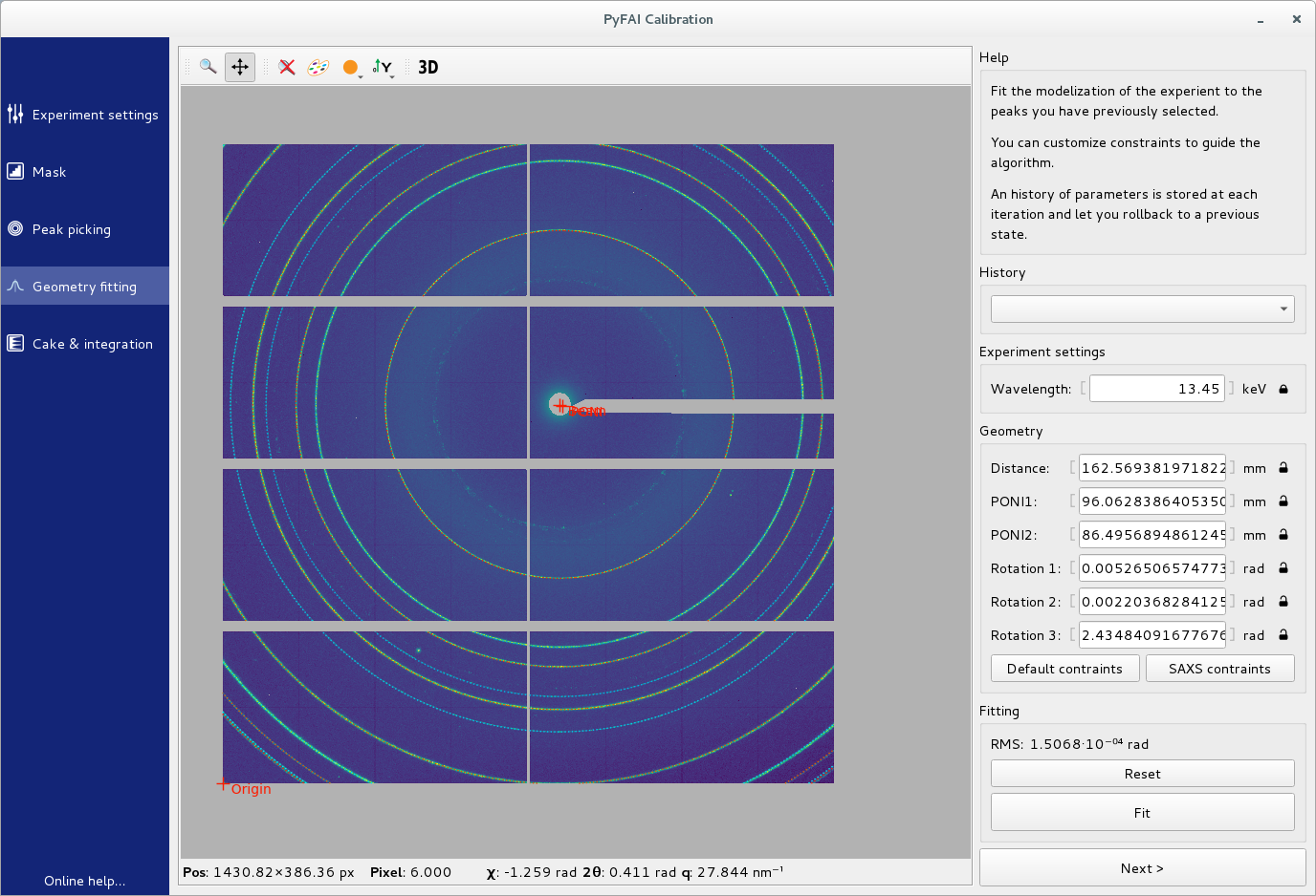
Values can be modified and fixed by clicking on the lock.
Click on the Fit button to re-fit the geometry.
Results may be displayed in various units by right-clicking on the unit.
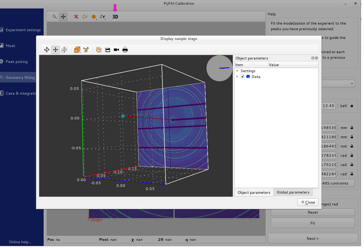
3D rendering#
As soon as a geometry is computed, it can be displayed as a 3D rendering. This view is available from the fitting screen, as a dedicated dialog box.
It uses the internal modelization of pyFAI: each pixel of the detector is spatialized. It textures them using the mask and the calibration image.
The beam is displayed a red cylinder smaller than the detector pixel size. It hits a symbol of the sample on one side, and according to the geometry can hit the detector on the other side.
Automatic peak-extraction#
Depending on the result, one may want to come back on the Peak picking task to
re-assign the ring numbers or select different peaks.
Or if it looks good, extracting many rings will allow for a more reliable fit.
For this, set the number of rings in the Recalibrate part and click Extract,
like in this figure:
The selected peaks with their ring assignment can be exported at this stage,
by clicking on the floppy disk icon.
This is used in the case of a goniometer calibration.
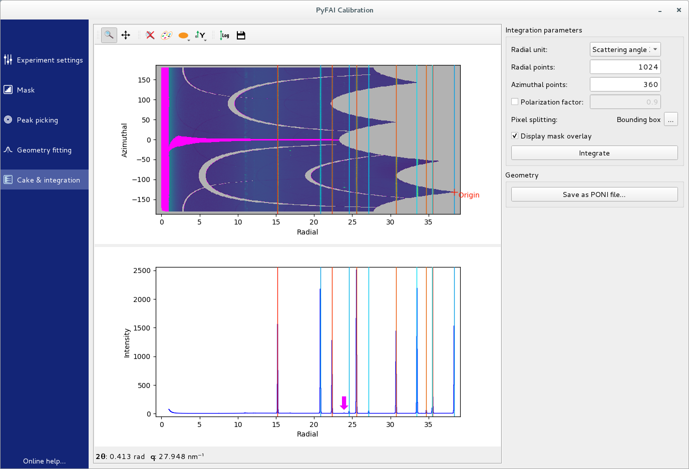
Cake and Integration#
The last task displays the 1D and 2D integrated image with the ring position overlaid to validate the quality of the calibration.
The radial unit can be customized and the images/curves can be saved.
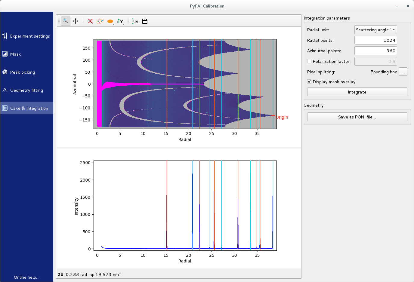
Last but not least, do not forget to save the geometry as a PONI-file for subsequent integrations.
Feedback from integrated result to improve the mask#
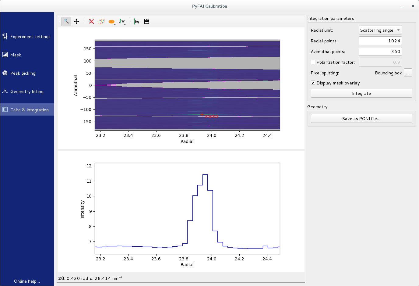
The 1D integration result can be used to notice misplaced peaks coming from hot pixels.
Once this hot pixel is located on the 1D spectrum, use the 2D view to localize it, then mark it using the right mouse button.
Back to the mask task.
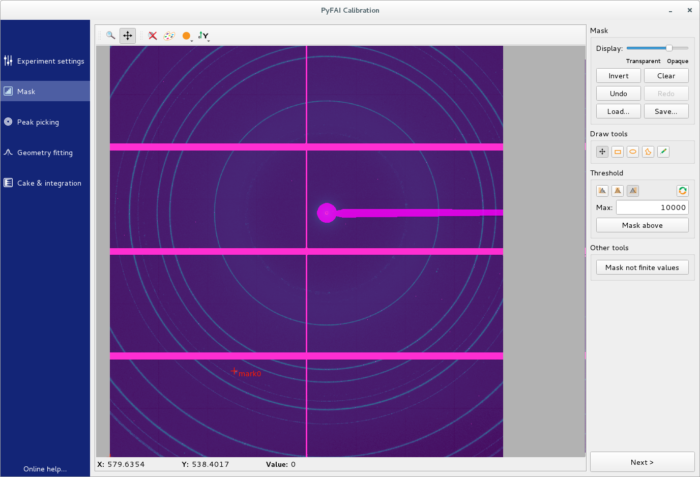
Zoom onto the mark.
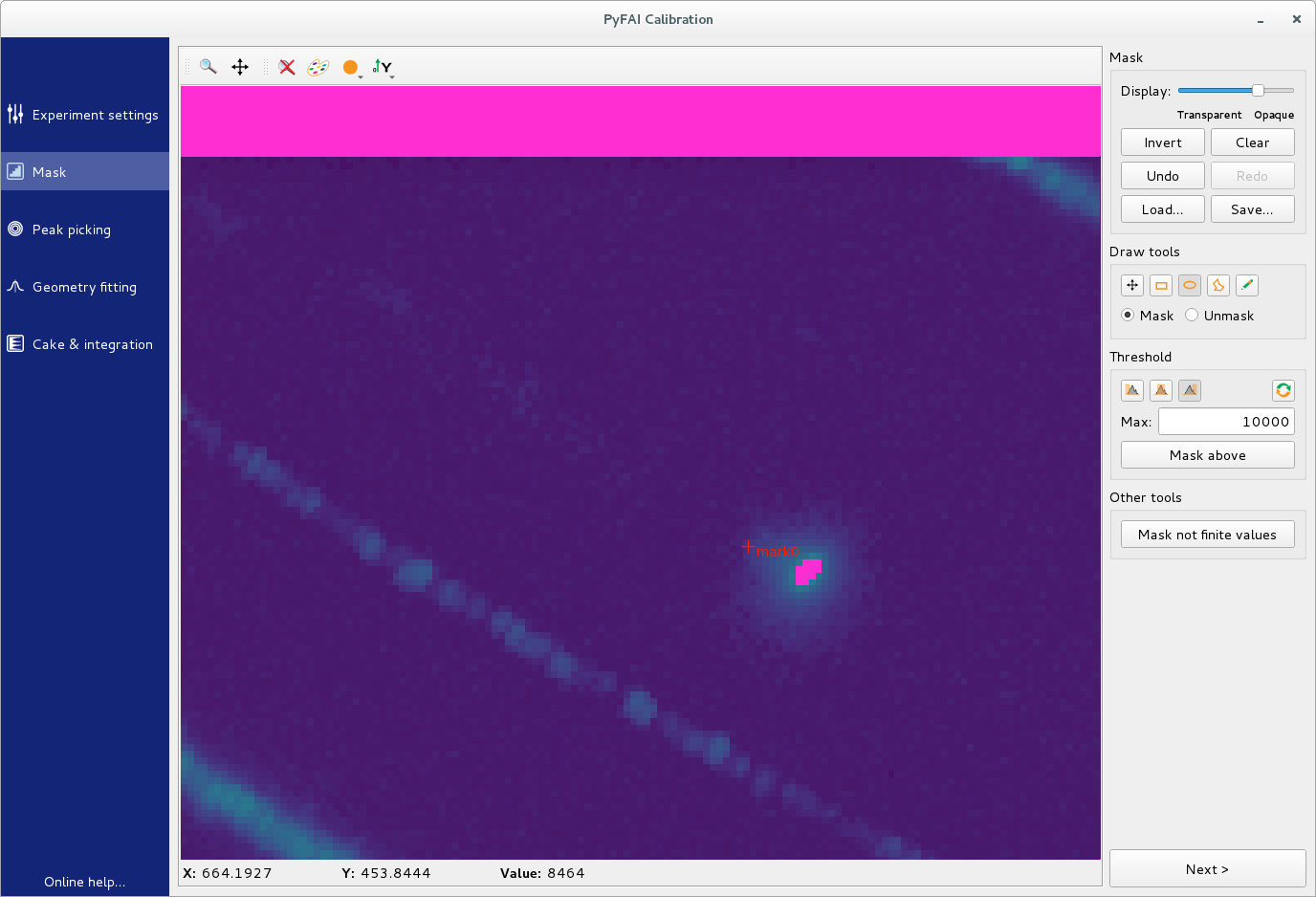
You can mask the defective area using one of the mask tools.
Back to the integration task, the result will be updated.
Conclusion#
This tutorial explained the 5 steps needed to perform the calibration of the detector position prior to any diffraction experiment on a synchrotron.
Advanced video tutorial#
This tutorial was given at the Hercules courses in 2020, the data files used are here: Calibration_Al2O3.h5 and kevlar.h5. This 65mn tutorial presents also silx view, pyFAI-average and pyFAI-integrate.